My first speedy forecast

Short description of the SPEEDY model

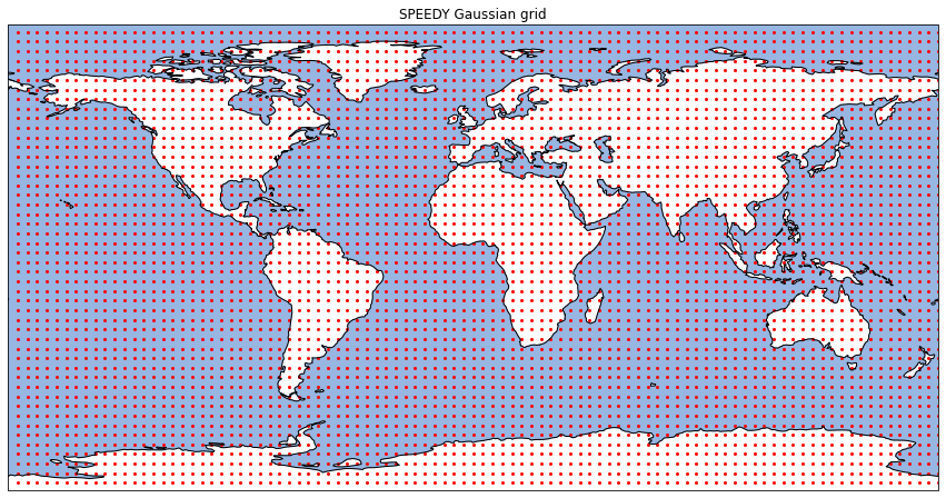
SPEEDY is an atmospheric global circulation model that uses the spectral dynamical core developed at the Geophysical Fluid Dynamics Laboratory. Its main characteristics are: - A spectral-transform model in the vorticity-divergence form with a semi-implicit treatment of gravity waves. - Hydrostatic σ-coordinate in the vertical coordinate. - The principal model prognostic variables are vorticity, divergence, temperature, and the logarithm of surface pressure. - Humidity is advected by the dynamical core, and with its sources and sinks are determined physical parametrizations. - The horizontal resolution corresponds to a triangular spectral truncation at total wavenumber 30 (T30, approximately 3.75 x 3.75 degree resolution). This corresponds to a Gaussian grid of 96 (longitude) by 48 (latitude) points. - For the vertical coordinate, eight levels are used with boundaries at σ values of 0, 0.05, 0.14, 0.26, 0.42, 0.60, 0.77, 0.90 and 1. The prognostic variables (except log(ps)) are specified at the σ levels in between the latter boundaries, namely at σ 0.025, 0.095, 0.20, 0.34, 0.51, 0.685, 0.835 and 0.9 - Time step: 40min. That is, 36 time steps per day.

For additional details, check the SPEEDY documentation here.

The boundary conditions

The boundary conditions needed to run SPEEDY are:

• Time invariant fields (lon, lat):

  • orog: Orographic height [m]

  • lsm: Land sea mask fraction. Values between 0 and 1.

  • vegl: Low vegetation cover (fraction). Values between 0 and 1.

  • vegh: High vegetation cover (fraction). Values between 0 and 1.

  • alb: Annual-mean albedo (fraction). Values between 0 and 1.

• Monthly-average climatological fiel for each month of the year (lon, lat, month):

  • stl: Land surface temp (top-layer) [degK].

  • snowd: Snow depth [kg/m2]

  • swl1: Soil wetness (layer 1) [vol. fraction, 0-1]

  • swl2: Soil wetness (layer 2) [vol. fraction, 0-1]

  • swl3: Soil wetness (layer 3) [vol. fraction, 0-1]

  • icec: Sea-ice concentration (fraction). Values between 0 and 1.

  • sst: Sea surface temperature [degK].

• Anomaly fields (lon, lat, day):

  • ssta: Sea surface temperature anomaly [degK].

The exact shapes for the invariant fields are (lon, lat, month) = (96, 48, 12). In contrast, the anomaly field (SST anomaly) needs to be provided for each day of the simulation period. For example, for a one-month forecast (30 days), the shape of the anomaly field is (96, 48, 30).

By default, the pySPEEDY package includes the example boundary conditions initially included in the SPEEDY.f90 package. These fields were derived from the ERA-interim re-analysis using the 1979-2008 period. In addition, the default boundary conditions include the monthly SST anomalies for the 1979-01-01 to 2013-12-01 period.

The initial conditions

The current version of pySPEEDY initializes all spectral variables at a reference atmosphere at rest with the following properties: Troposphere: T = 288°K at the surface. Constant temperature lapse rate. Stratosphere: T = 216 °K, lapse rate = 0. Pressure field consistent with the temperature field. Humidity: qv = RHref * q_saturation(288K, 1013hPa) with RHref=0.7. For this initialization, the following spectral variables are initialized: - “vor [mx, nx, levels, 2]”: Vorticity in the spectral space. Complex. - “div [mx, nx, levels, 2]”: Divergence in the spectral space. Complex. - “t [mx, nx, levels, 2]”: Temperature in the spectral space. Complex. - “ps [mx, nx, 2]”: Log of (normalised) surface pressure. - “phi [mx, nx, levels]”: Atmospheric geopotential. Real. - “phis [mx, nx]”: Surface geopotential. Real. - “tr [mx, nx, levels, 2, ntr]”: Tracers. Currently, it only contains humidity. Real.

where mx=31, nx=32, levels=8, ntr=1 (number of tracers). The “2” in the last dimension indicates that the variable is complex (0-real/1-imaginary).

Google colab fix

IMPORTANT

If you are running this notebook in Google Colab, uncomment and execute the following lines to install pySPEEDY and its dependencies.

# !apt-get install libproj-dev proj-data proj-bin
# !apt-get install libgeos-dev libnetcdf-dev libnetcdff-dev

# !pip uninstall --yes shapely
# !pip install shapely --no-binary shapely
# !pip install cartopy

Temporary fix for https://github.com/SciTools/cartopy/issues/1869 proposed by @rcomer

# !wget https://raw.githubusercontent.com/SciTools/cartopy/master/tools/cartopy_feature_download.py
# !python cartopy_feature_download.py physical

Now we install pySPEEDY

#!pip install -v git+https://github.com/aperezhortal/pySPEEDY.git

End of Colab setup.

My first forecast

Let’s run our first forecast. In the following example we will run the forecast for 3 months starting from a rest atmosphere. The first month will be considered as the model spinup period over which the model outputs are not saved.

%%time
from datetime import datetime

from pyspeedy import Speedy
from pyspeedy.callbacks import ModelCheckpoint, XarrayExporter

start_date = datetime(1980, 1, 1)  # Simulation start date (datetime object).
end_date = datetime(1980, 2, 29)  # Simulation end date.
spinup_date = datetime(1980, 2, 1)  # End of spinup period.

# Create an instance of the speedy model.
model = Speedy(
    start_date=start_date,  # Simulation start date (datetime object).
    end_date=end_date,  # Simulation end date.
    diag_interval=180,  # Every how many time steps we will compute the diagnostics.
)
# At this point, the model state is "empty".

# To initialize the model, we need to define its boundary conditions first.
# This function will set the default boundary conditions derived from the ERA reanalysis.
model.set_bc()

# Before running the model, let's initialize two callback functions that

# Initialize the callback functions that saves the model data into netcdf files
# A "callback" is an object that performs user defined actions at each time step.
my_exporter = XarrayExporter(
    output_dir="./data",  # Output directory where the model output will be stored
    interval=36,  # Every how many time steps we will save the output file. 36 -> once per day.
    verbose=True,  # Prind progress messages
    variables=None,  # Which variables to output. If none, save the most commonly used variables.
    spinup_date=spinup_date,  # End of spinup period
)

# Let's initialized another callback. This one keeps a dataframe with selected variables
# with different model times ("checkpoints").
# The dataframe with the data is stored in the "dataframe" attribute of the
# create ModelCheckpoint instance.
model_checkpoints = ModelCheckpoint(
    interval=36,  # Every how many time steps we will save the output file. 36 -> once per day.
    verbose=True,  # Prind progress messages
    variables=None,  # Which variables to output. If none, save the most commonly used variables.
    spinup_date=spinup_date,  # End of spinup period
)


# Print the names of output variables that will be saved.
# Note that the variables shown next are in the grid space (not the spectral space)
print("Exported variables:")
print(my_exporter.variables)

# Run the model. We pass the a list of callbacks
model.run(callbacks=[my_exporter, model_checkpoints])
# After the model is run, the model state will keep the last values of the last integration step.

Exported variables:
('u_grid', 'v_grid', 't_grid', 'q_grid', 'phi_grid', 'ps_grid')
Saving model output at: ./data/1980-02-01_0000.nc.
Saving model output at: ./data/1980-02-02_0000.nc.
Saving model output at: ./data/1980-02-03_0000.nc.
Saving model output at: ./data/1980-02-04_0000.nc.
Saving model output at: ./data/1980-02-05_0000.nc.
Saving model output at: ./data/1980-02-06_0000.nc.
Saving model output at: ./data/1980-02-07_0000.nc.
Saving model output at: ./data/1980-02-08_0000.nc.
Saving model output at: ./data/1980-02-09_0000.nc.
Saving model output at: ./data/1980-02-10_0000.nc.
Saving model output at: ./data/1980-02-11_0000.nc.
Saving model output at: ./data/1980-02-12_0000.nc.
Saving model output at: ./data/1980-02-13_0000.nc.
Saving model output at: ./data/1980-02-14_0000.nc.
Saving model output at: ./data/1980-02-15_0000.nc.
Saving model output at: ./data/1980-02-16_0000.nc.
Saving model output at: ./data/1980-02-17_0000.nc.
Saving model output at: ./data/1980-02-18_0000.nc.
Saving model output at: ./data/1980-02-19_0000.nc.
Saving model output at: ./data/1980-02-20_0000.nc.
Saving model output at: ./data/1980-02-21_0000.nc.
Saving model output at: ./data/1980-02-22_0000.nc.
Saving model output at: ./data/1980-02-23_0000.nc.
Saving model output at: ./data/1980-02-24_0000.nc.
Saving model output at: ./data/1980-02-25_0000.nc.
Saving model output at: ./data/1980-02-26_0000.nc.
Saving model output at: ./data/1980-02-27_0000.nc.
Saving model output at: ./data/1980-02-28_0000.nc.
Saving model output at: ./data/1980-02-29_0000.nc.
CPU times: user 44.5 s, sys: 328 ms, total: 44.8 s
Wall time: 44.7 s

The time series of the selected variables are stored in a dataframe inside the model_checkpoints object that we pass as a callback to the model run.

# Check the stored dataframe in the model checkout callback.
model_checkpoints.dataframe

<xarray.Dataset>
Dimensions:  (time: 29, lev: 8, lat: 48, lon: 96)
Coordinates:
  * time     (time) datetime64[ns] 1980-02-01 1980-02-02 ... 1980-02-29
  * lev      (lev) float32 0.95 0.835 0.685 0.51 0.34 0.2 0.095 0.025
  * lon      (lon) float32 0.0 3.75 7.5 11.25 15.0 ... 345.0 348.8 352.5 356.2
  * lat      (lat) float32 -87.22 -83.51 -79.79 -76.08 ... 79.79 83.51 87.22
Data variables:
    u        (time, lev, lat, lon) float32 -1.161 -0.8675 -0.572 ... 2.781 2.537
    v        (time, lev, lat, lon) float32 -3.48 -3.515 -3.519 ... -5.552 -5.649
    t        (time, lev, lat, lon) float32 247.6 247.2 246.9 ... 192.4 192.3
    q        (time, lev, lat, lon) float32 0.0003778 0.0003718 ... 0.0 0.0
    phi      (time, lev, lat, lon) float32 3.119e+03 3.176e+03 ... 2.304e+04
    ps       (time, lat, lon) float32 7.234e+04 7.178e+04 ... 1.023e+05

Note that the dimensions in the dataframe were reordered to follow the conventions typically used in NWP model outputs. This ordering differs from the internal dimension ordering use by the the underlying SPEEDY.90 (state variables).

For convenience, all the state variables in the SPEEDY.90 model can be accessed from python using items getters and setters.

For example, the model latitude and longitude can be accessed as model["lat"] or model["lon"]. Similarly, to update the value of, let’s say, temperature in the grid space, we use: model[t_grid]=new_t_grid_array

A complete description of the state variables that can be accessed through python are listed in this table.

The model grid

Let’s plot the model grid first to visualize the model’s resolution.

import cartopy.crs as ccrs
import matplotlib
import matplotlib.pyplot as plt
import numpy as np
from cartopy.feature import OCEAN

fig = plt.figure(figsize=(15, 10))
ax = plt.subplot(projection=ccrs.PlateCarree())

longitude_2D, latitude_2D = np.meshgrid(model["lon"], model["lat"])
ax.set_title("SPEEDY Gaussian grid")  # Add title for each subplot.
ax.set_global()  # Set global extention
ax.coastlines()  # Add coastlines
ax.add_feature(OCEAN)  # Add oceans
_ = ax.scatter(
    longitude_2D, latitude_2D, s=4, c="red", marker="o", transform=ccrs.PlateCarree()
)

Matplotlib is building the font cache; this may take a moment.
/home/docs/checkouts/readthedocs.org/user_builds/pyspeedy/conda/latest/lib/python3.8/site-packages/cartopy/io/__init__.py:241: DownloadWarning: Downloading: https://naturalearth.s3.amazonaws.com/110m_physical/ne_110m_ocean.zip
  warnings.warn(f'Downloading: {url}', DownloadWarning)
/home/docs/checkouts/readthedocs.org/user_builds/pyspeedy/conda/latest/lib/python3.8/site-packages/cartopy/io/__init__.py:241: DownloadWarning: Downloading: https://naturalearth.s3.amazonaws.com/110m_physical/ne_110m_coastline.zip
  warnings.warn(f'Downloading: {url}', DownloadWarning)

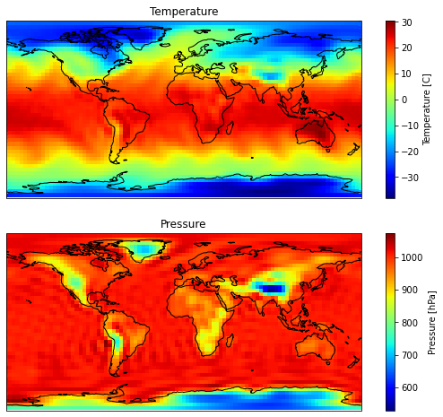
Now let’s plots some prognostic variables at the surface.

from cartopy.util import add_cyclic_point

# The shape of the t_grid field is ['lon', 'lat', 'lev']
# The vertical dimension is sorted in decreasing height.
# That means that the [:,:,0] indicates the highest level, while [:,:,1] indicate the lowest level.
# For the temperature field we will plot the lowest level (surface).
# The shape of the ps_grid is ['lon', 'lat']

variables_to_plot = [
    # (model_variable_name, variable long name)
    (
        "t_grid",
        "Temperature",
        "[C]",
    ),  # Surface temperature in Kelvin degrees (in the grid space).
    ("ps_grid", "Pressure", "[hPa]"),  # Surface pressure
]

fig, axs = plt.subplots(
    2, 1, subplot_kw=dict(projection=ccrs.PlateCarree()), figsize=(10, 8)
)

lon = model["lon"]
lat = model["lat"]

for i, (var, title, units) in enumerate(variables_to_plot):
    ax = axs[i]
    plt.sca(ax)

    ax.set_title(title)  # Add title for each subplot.
    ax.set_global()  # Set global extention
    ax.coastlines()  # Add coastlines
    ax.add_feature(OCEAN)  # Add oceans

    data_to_plot = model[var]
    if var == "t_grid":
        # data_to_plot has [lon, lat, lev] dimensions.
        data_to_plot = data_to_plot[:, :, -1]  # Keep the lowest level
        data_to_plot -= 273.15
    elif var == "ps_grid":
        data_to_plot /= 100

    # Copy the longitude=0 degrees data to longitude=360 to have continuous plots
    data_to_plot, lon = add_cyclic_point(data_to_plot, coord=model["lon"], axis=0)
    lat = model["lat"]
    cs = ax.pcolormesh(
        lon,
        model["lat"],
        data_to_plot.T,
        transform=ccrs.PlateCarree(),
        cmap="jet",
        shading="auto",
    )
    cbar = plt.colorbar(cs, label=f"{title} {units}")
_ = plt.subplots_adjust(wspace=0.05)

TO BE CONTINUED